This post is a continuation of an earlier post I made. If you have not read it, you can read that post here.

Analysis

I am using the same data used in my earlier post. The first step is to import the necessary packages: sfnetworks, igraph, tidygraph, and sf. The sfnetworks package can convert the sf object into a network object. It makes our analysis way much easier. The igraph and tidygraph packages are used to extract centrality measures of an intersection.

FloridaCounties009 = st_read("./newfolder/tl_2020_12009_roads.shp", quiet = TRUE)

#Define the desired projection
proj = "+proj=utm +zone=17 +ellps=GRS80 +towgs84=0,0,0,0,0,0,0 +units=m +no_defs +type=crs"
#Projecting the shapefile to the defined projection
FloridaCounties009Proj = st_transform(FloridaCounties009, crs = proj)

#Creating spatial object from the latitude and longitude 
#information in the FloridaCrashData
CrashLocations = FloridaCrashData %>% 
  select(COUNTYNAME, LONGITUD, LATITUDE, TWAY_ID, TWAY_ID2, YEAR) %>% 
  filter(grepl("BREVARD", COUNTYNAME, ignore.case = TRUE)) %>% 
  st_as_sf(., coords = c('LONGITUD', 'LATITUDE'), crs = 4269)

I have selected the BREVARD county for the illustration purpose. Firstly, let’s import the shapefile of that county’s road networks. Followed by transforming the shapefile into the desired projection. Finally, I extracted the latitude and longitude information and converted them into an sf object.

# Create the igraph of road networks using sfnetworks package
g <- as_sfnetwork(x = FloridaCounties009, 
                              directed = FALSE, 
                              length_as_weight = TRUE, 
                              edges_as_lines = TRUE)
g <- g %>%
  activate("nodes") %>% 
  mutate(BetweennessCentrality = centrality_betweenness(
    weights = weight, normalized = TRUE, 
    directed = FALSE)) %>%
  mutate(DegreeCentrality = centrality_degree(normalized = TRUE) )

Here, I use the sfnetwork package to create a network object from the shapefile I imported. The network object is stored in the variable g. At this point we can calculate any centrality measures of an intersection. As an example, I calculated centrality_betweenness and centrality_degree. You can calculate any desired network measures at this stage. Let’s look at the distribution of Degree Centrality measure.

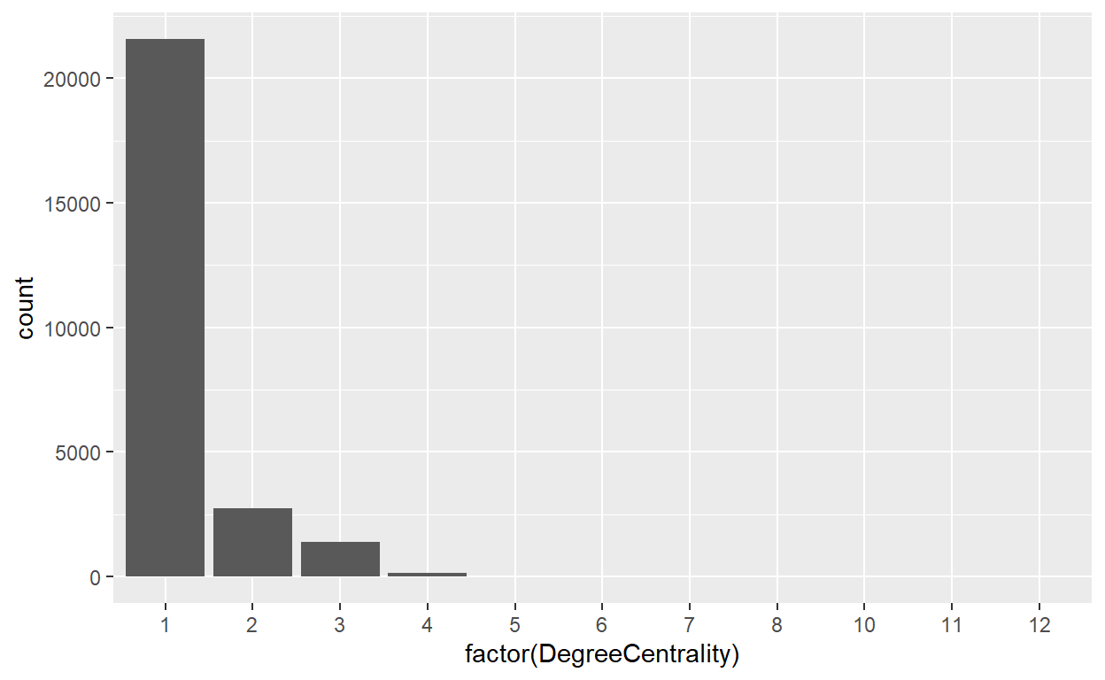
It seems that there are more dead ends (degree of 1 means dead ends). It is a bit off to have this many dead ends. I think the sfnetworks is not performing well. Let’s not dwell in this for now as we are not interested in that. Now, we can extract teh location of each intersection using the following code. One thing to notice here is that when we are interested in nodes, we need to activate nodes first. If you are interested in edges, you need to activate edges first then perform the analysis.

#Extract the all intersection coordinates from the graph
node_coords <- g %>% activate("nodes") %>% 
  st_coordinates() %>% as.data.frame %>% 
  st_as_sf(coords = c("X","Y"), crs = 4269) 

#Extract the location of crashes
crash_points <- CrashLocations %>% st_coordinates() %>% 
  as.data.frame %>% 
  st_as_sf(coords = c("X","Y"), crs = 4269)

We extracted all the points of intersections from the network object, and all points (location) of crash sites. Now, for a give crash site location, We can calculate the distance between that crash location and all intersection points. Then we can arrange them in ascending order and pick the first value and the index of the node (i.e. intersection).

#Identifying the closest intersections based on computing distance
ind_ <- c()

for(i in 1:length(crash_points$geometry)) {
  d <- st_distance(crash_points$geometry[i], node_coords$geometry)
  ind_ <- c(ind_, which(d == min(d))) }

Here, I have extracted all the indices of intersections that are closest to the crash locations.

# Extract the intersection points
crash_points <- cbind(ind_, crash_points)  
IntersectionsNearCrashPoints <- node_coords %>% slice(ind_) %>% 
  st_transform(., crs = proj)

Let’s plot them and see. The green dots are crash location and red squares are the intersection closest to a crash location.

#Plotting the crash locations and intersections near crash locations
tm_shape(FloridaCounties009Proj) + tm_lines() +
  tm_shape(CrashLocations) + tm_dots(size = .1, col = 'green') +
  tm_shape(IntersectionsNearCrashPoints) + tm_dots(shape = 0, 
                                                   size = .1, col = 'red')

Et Voilà! That’s it for this post. Once we have the intersection information i.e. latitude and longitude, closest to the crash site, we can find many road network information specific to that crash location. This information can be integrated in our analyses to make accurate prediction (or inferences).

Analysis of Fatal Traffic Crashes in Florida: Part 2

Analysis

Corrections